The post takes a half-technical tone, assuming the reader is familiar with math at a post-high school level.

Although there are great explanations of AIXI, such as this one (to which I owe immense credit), I wanted to give a go at writing a technical explanation of it, and explained aspects of AIXI that I would have appreciated while learning about it.

Recently, AI has undergone a dramatic phase change. AI systems have become significantly more capable in various domains, and it feels as though our modern systems have reached a qualitatively ‘higher’ level of intelligence.

How can we quantify this intelligence? It’s difficult; neuroscientists and AI researchers have been thinking about this for years. While they have gotten close, the best we have are toy models. This blog post will introduce one of the earliest, most intuitive toy models: AIXI.

AIXI, along with other reinforcement-learning-esque approaches towards defining intelligence, focuses instead on describing goal-directed systems, a notion far more natural. When formulating a definition of intelligence, if we instead focus on the end goal of maximizing a reward/utility/number rather than trying to flush out the messy specifics of intelligence, we can make much more progress!

The central question is thus, “How do we maximize reward”? Reinforcement Learning has developed many approaches towards this, but AIXI is an early, famous toy model formulated to achieve this on a superhuman scale.

The Environment

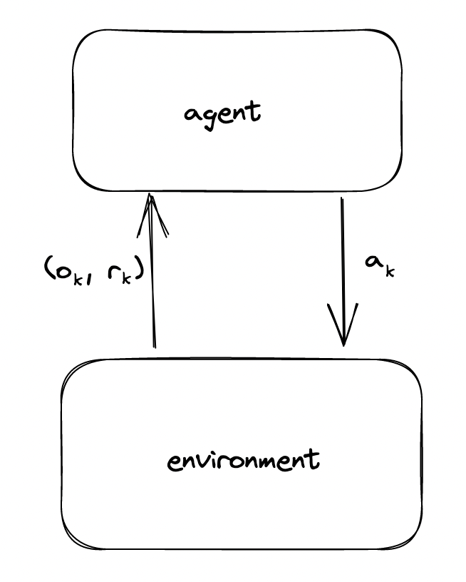
The setting for AIXI is intuitive. There is an agent and an environment - two distinct, separate entities - which interact sequentially over the course of $m$ timesteps. At time step $t$, the agent provides an action $a_t$ to the environment, and in response, the environment reacts with an observation $o_t$ and reward $r_t$ ¹. This observation and reward is fed back into the agent, who then uses the new information to provide a new action.

While the specifics of actions and observations are abstract and ignorable, for the sake of this discussion, we can assume that all actions $a_t \in A$ and observations $o_t$ are discrete objects, and all rewards $r_t \in R$ are real numbers. The goal, thus, is to maximize the total reward $r_1 + r_2 + … + r_m$.

The environment is computable and deterministic. Although it is formally a Turing Machine, we can identically model it as a function $E$, which maps from a history (string) of actions, observations, and rewards to a new observation and reward

$$E(a_1o_1r_1a_2o_2r_2…o_{k-1}r_{k-1}a_k) = (o_k,r_k)$$ Notice that since the environment is deterministic, we could also model the environment as $$E(a_1a_2…a_{k-1}) = (o_k,r_k)$$ Although the environment is deterministic, the agent’s understanding of it is probabilistic - it does not have a perfect understanding of the environment. As such, rather than modeling the environment with the deterministic function $E$, the agent instead will model the environment stochastically as a probability distribution $\mu(o_kr_k|a_1o_1r_1…r_{k-1}o_{k-1}a_k)$.

Readers here familiar with Reinforcement Learning should notice that there is no Markov Assumption with this environment - the past history is used in determining the next observation and reward.

The Agent

At this point, we have an environment - a source of rewards and observations - and a notion of the agent, which provides actions to the environment. Now, we must get to the hard part of specifying how the agent chooses actions. Recall that our agent should choose actions that maximize $\sum_{1}^m{r_k}$.

Formally, AIXI chooses its actions as follows; don’t worry, we’ll walk through the equation step by step. It’s a bit overwhelming. $$a_{t}:=\underset{a_t}{argmax}\left(\sum_{o_{t}r_{t}}\ldots \left(\underset{a_m}{max}\sum_{o_{m}r_{m}}[r_{t}+\ldots +r_{m}]\left(\sum_{q:;U(q,a_{1}\ldots a_{m})=o_{1}r_{1}\ldots o_{m}r_{m}}2^{-{{length}}(q)}\right)\right)\right)$$

Let’s forget about all of that and work our way up to this equation.

Let’s start with a toy environment. You are driving a car and have three possible actions: at each time step, you can take an action $a_k \in A = {up, down, forward}$. You’ve just received an observation and reward, $r_{k-1}=10$ , depicted below.

For each possible action, you happen to know eactly what the next reward and observation wil be.

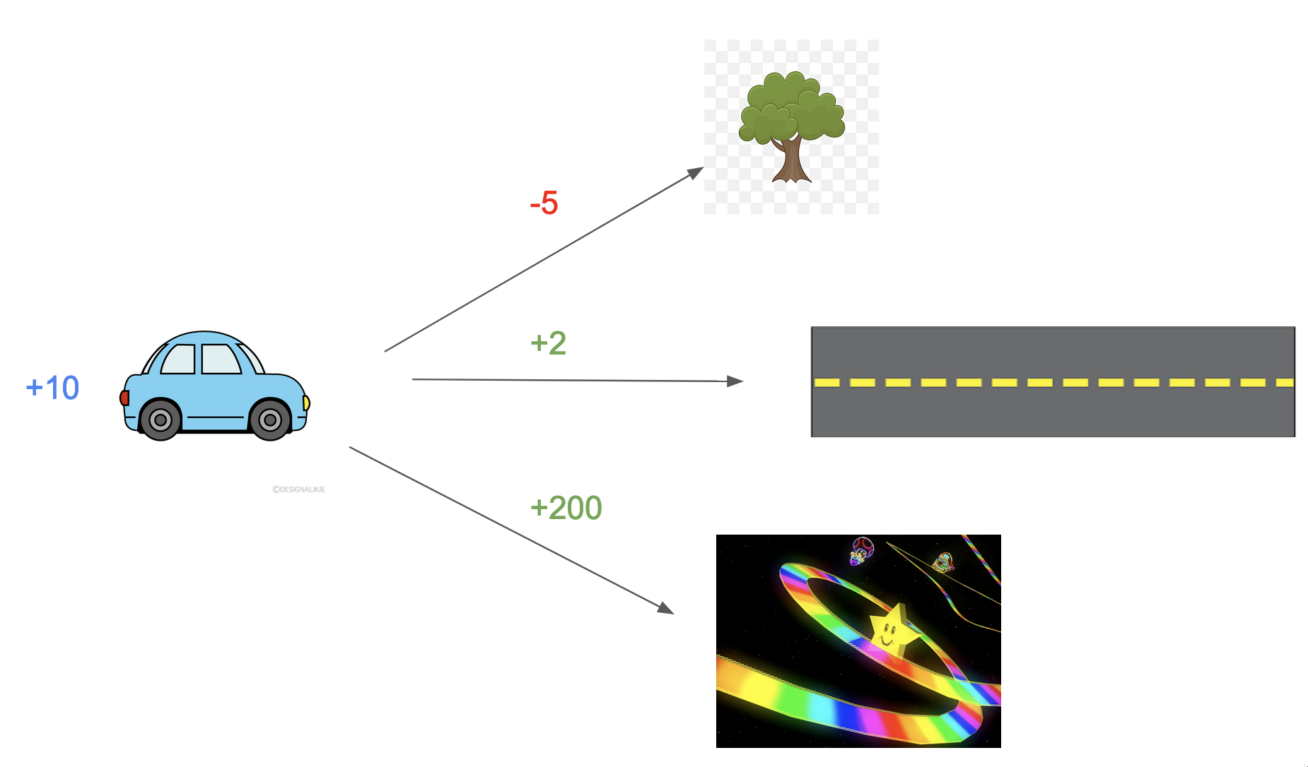
In this instance, what action should you choose? This is trivial - simply pick the action that gives you the highest reward! You know that the going downwards into Rainbow Road gives you the most reward, and would choose to go downwards. In general, in situations analogous to this, you would pick the action according to this general heuristic:

$$a_k = \underset{a_k \in A}{\arg\max} \ E({r_k | a_k}) $$

[!Note] Quick notation note: for simplicity sake, we will assume that all probabilities takes into account all past history beyond what is written. So, if we write $\mu(…|a_ko_kr_k)$, this is $\mu(…|a_1o_1r_1…a_ko_kr_k)$; similarily, above, $E(r_k|a_k)$ is really $E(r_k|a_1o_1r_1…a_k)$

Notice how we’ve formulated the equation in terms of expected reward. In this above toy scenario, we know what rewards an action will yield; however, most of the time, we don’t precisely know what reward we will get from taking an action, but instead have a probability distribution over possible rewards.

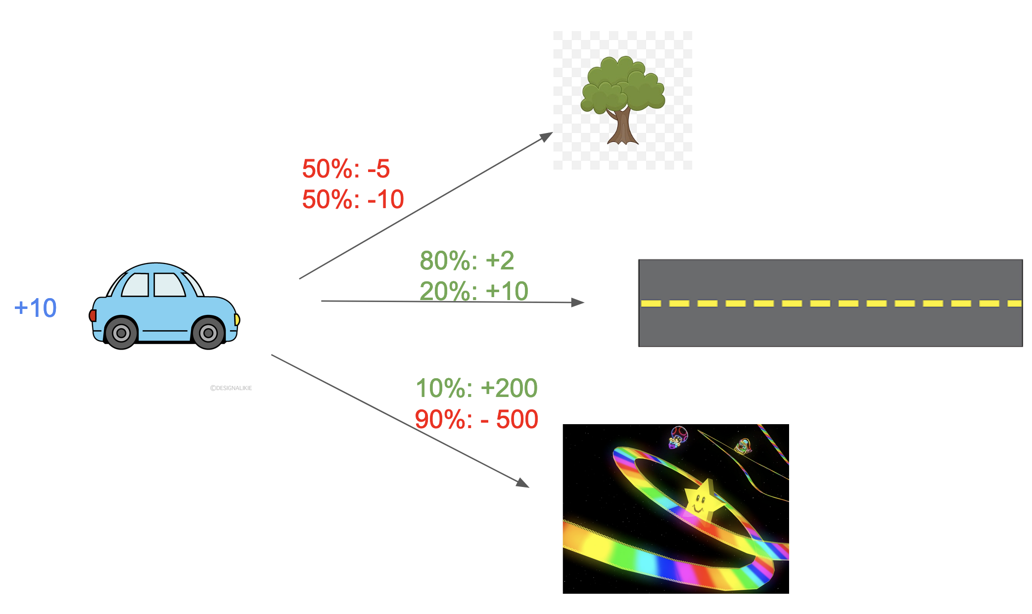
Now our toy scenario holds probabilities. This is a much more realistic notion of our environment! Here, we would pick the action according to highest expected reward. And indeed, when working with AIXI, we have a probabilistic model of possible rewards we will receive from taking an action - recall that our Agent models a probability distribution $\mu$ of the environment.

We can write this as:

$$a_k = \underset{a_k \in A}{\arg\max} \ E({r_k | a_k}) = a_k =\underset{a_k \in A}{\arg\max} \ \sum _{o_k \in O, r_k \in R} (r_k)\mu(o_kr_k|a_k) $$ (where $R$ is the set of all possible rewards, $O$ is the set of all possible observations, and $\mu$ is the agents current probability distribution of the environment.)

In our above toy scenario, the best option is to go towards the middle, as it has the highest expected reward $(0.8)2 + (0.2)10 = 3.6$

Looking Into The Future

While this approach is a decent start, it is considered greedy - it only focuses on the immediate next reward and doesn’t plan long-term. Our goal is to maximize $r_1 + r_2 + … + r_m$, not just the next time step!

We thus need to extend this equation to allow the agent to model over multiple steps. As such, when our agent selects an action at $a_k$, it should also be thinking about the potential actions it would take at actions $a_{k+1}, a_{k+1}, …., a_m$.

Let’s update the above toy scenario, and imagine we are trying to plan over two timesteps. 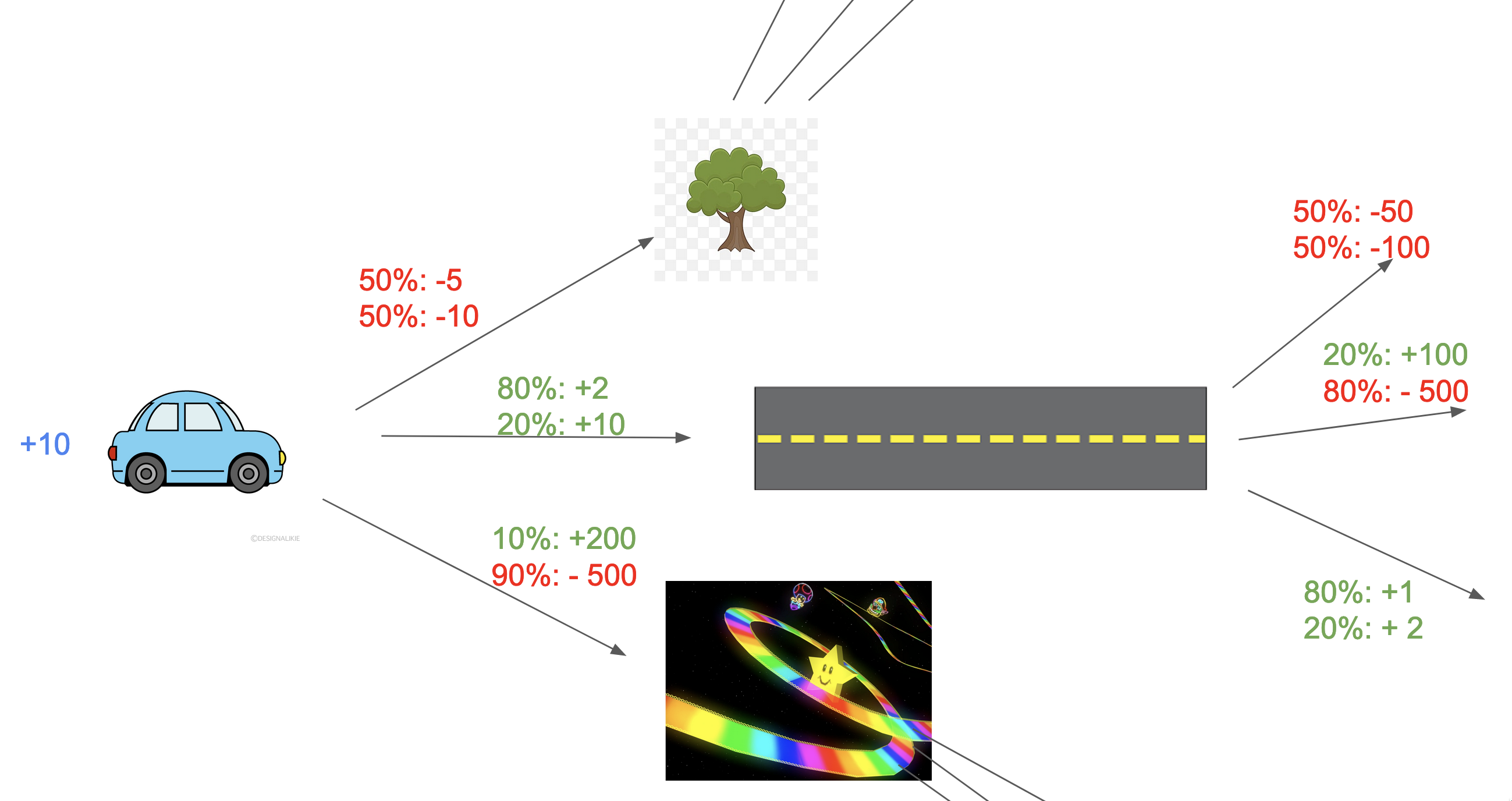When evaluating the first possible action, it needs to consider both the direct reward from the action, as well as the expected reward at the following timestep. So, on top of what we had earlier, we now add:

$$a_k = \underset{a_k \in A}{\arg\max} \ \sum_{o_k \in O, r_k \in R} (r_k \color{yellow}+ E(r_{k+1}|a_ko_kr_k)\color{white})\mu(o_kr_k|a_k) $$ Intuitively, what will this new expected value to be? Say we have gone forwards on the normal road: it’s not as though our next action is probabilistic. It would be downwards, as it has the highest expected reward of $E(r_{k+1}|forward,road,3.6,down)=(.8)1 + (.2)2 = 1.2$!

Similarly, in our general formulation, our second action is chosen based of another mathematical prediction of the action which yields the highest expected reward²!

$${\displaystyle E(r_{k+1}|a_ko_kr_k) = \underset{a_{k+1}}{max}\left( \sum_{o_{k+1}\in O,r_{k+1} \in R}{} r_{k+1}\mu(o_{k+1}r_{k+1}|a_ko_kr_ka_{k+1})\right)}$$

Before we expand this expected value, we can move the $r_k$ inside the expected value, as it stays constant throughout the scope of the summation. $$a_k = \underset{a_k \in A}{\arg\max} \ \sum_{o_k \in O, r_k \in R} E(r_k + r_{k+1}|a_ko_kr_k)\mu(o_kr_k|a_k) $$ What is this new expected value? Analogously to the above, its the expected value of highest predicted ‘sum of of rewards’.

$$E(r_k + r_{k+1}|a_ko_kr_k) = \color{orange}\underset{a_{k+1}}{max} \sum_{o_{k+1} \in O, r_{k+1} \in R} (r_k + r_{k+1})\mu(o_{k+1}r_{k+1}|a_ko_kr_ka_{k+1})$$

We can now plug this in and further multiply the term $\mu(o_kr_k|a_k)$ through the inner sum

$$a_k = \underset{a_k \in A}{\arg\max} \ \sum_{o_k \in O, r_k \in R} \color{orange}\underset{a_{k+1}}{max} \sum_{o_{k+1} \in O, r_{k+1} \in R} (r_k + r_{k+1})\mu(o_{k+1}r_{k+1}|a_ko_kr_ka_{k+1})\color{white}\mu(o_kr_k|a_k) $$

Now we perform a bit of a dubious substitution³, asserting that future actions don’t give new information on past experiences, such that $\mu(o_kr_k|a_k) = \mu(o_kr_k|a_ka_{k+1})$. If we do that, we can then multiply $$\mu(o_{k+1}r_{k+1}|a_ko_kr_ka_{k+1})\mu(o_kr_k|a_k) = \mu(o_{k+1}r_{k+1}|a_ko_kr_ka_{k+1})\mu(o_kr_k|a_ka_{k+1}) = \mu(o_kr_ko_{k+1}r_{k+1}|a_ka_{k+1})$$ and plug this all back into the original equation to get a more natural, understandable equation:

$$a_k = \underset{a_k \in A}{\arg\max} \ \sum_{o_k \in O, r_k \in R} \underset{a_{k+1}}{max} \sum_{o_{k+1} \in O, r_{k+1} \in R} (r_k + r_{k+1})\mu(o_kr_ko_{k+1}r_{k+1}|a_ka_{k+1}) $$

You can now just intuitively imagine this as completing an expected value calculation over two time steps, while also adding an implicit assumption that the model will act optimally.

Maxing all the way

Now approach this generalizes all the way to $m$ timesteps

$$a_{k}:=\arg \max_{a_{k}}\left(\sum_{o_{k}r_{k}}\underset{a_{k+1}}{max}\ldots \left(\max_{a_{m}}\sum_{o_{m}r_{m}}[r_{t}+\ldots +r_{m}]\mu(o_kr_k…o_mr_m|a_ka_{k+1}…a_m)\right)\right)$$

We have an equation that completes an expected total reward calculation over $m-k$ timesteps, weaving in the assumption that the model continues to act optimally.

This is almost the final AIXI equation. The last piece of magic deals with the probability distribution $\mu$!

Making Priors From Nothing But Programs

We’ve been throwing around this probability distribution $\mu$ as if it is given to us, but in reality, we must derive it. If it was given, this would be a relatively trivial problem! Indeed, much of the difficulty comes in learning this probability distribution. Formulating this prior, especially from nothing, is not trivial.

The following will be a rushed, hopefully intuitive, explanation of the Komogorov Complexity and Solomonoff Prior.

When creating the starting prior for our probability distribution, we can follow a general notion that simpler explanations are more likely to be true - see Occams Razor for more intuition behind this. AIXI uses this to generate the Solomonoff Prior, which takes this premise, formalizes it, and runs with it.

Compare the following two products of a random string generator, 000000000000 and 101000101000. Of course, if you were to request a random binary string of length 12, both of these would be equally likely. But do they appear equally random? No! The first string appears to be repeated 0s, and the latter just looks like… nonsense, true ‘randomness.’

When looking at these strings, we have this sense that one is more ‘complicated’ than the other. This ‘complexity’ is essential, and we can capture this intuition by thinking about how long it would take a software program to describe the strings.

For instance, perhaps you could easily describe the first string in Python as print("0" * 12) - a really short program! But the other string? There’s not a super convenient way to compress it! Perhaps the shortest computer program would just store the string itself, print(101000101000).

This is similar to how Komogorov Complexity operates. Given an observation, it is the simplest possible program which could give rise to an observation. Data is produced from programs - and for each program, we can create a ’length’ for it, denoted as $l(x)$, which acts as an metric for us to describe its complexity⁴.

AIXI doesn’t just look at the simplest program which could produce an observation, but rather all possible ones.

Put yourself back in AIXI-space; imagine we have a history of observations, rewards, and actions that have occured. Let’s say that x is one possible program that could have outputted these observations and rewards. It’s Komogorov Length would be $l(x)$, and the Solomonoff Prior asserts that, a priori,

$$P(E=x) = 2^{-l(x)}$$ AIXI uses this solomonoff prior for its probability distribution $\mu$. Thus, when calculating the value of different probability distributions in $\mu$, we can sum over all possible programs which could produce the series of observations, rewards, and actions!

$$\mu(o_kr_k…o_mr_m|a_ka_{k+1}…a_m) = \sum_{x:;U(x,a_{1}\ldots a_{m})=o_{1}r_{1}\ldots o_{m}r_{m}}2^{-{\textrm {length}}(x)}$$ (where $U$ is a monotone universal Turing machine, and x is a possible program)

It’s important to note that The Solomonoff Prior is incomputable, which is why AIXI is also incomputable.

Putting it All Together

And, as a result, we end up with our final equation

${\displaystyle a_{t}:=\arg \max_{a_{t}}\left(\sum_{o_{t}r_{t}}\ldots \left(\max_{a_{m}}\sum_{o_{m}r_{m}}[r_{t}+\ldots +r_{m}]\left(\sum_{q:;U(q,a_{1}\ldots a_{m})=o_{1}r_{1}\ldots o_{m}r_{m}}2^{-{\textrm {length}}(q)}\right)\right)\right)}$

All at once, this is:

• calculating expected rewards over all possible actions
• assigning probabilities precisely according to Occams Razor and the Solomonoff Prior
• assuming that the agent is acting optimally

AIXI serves as a really good toy model for understanding how intelligence works! Lots of exciting properties about AIXI have been proven, and it serves as a good starting point for thinking about intelligence.

While AIXI helps study intelligence, it has various limitations that prevent this from being a basis for implementing real-world superintelligence. Importantly, there is the obvious issue that it is incomputable (although there have been approximations to AIXI which have been successfully implemented)

Additionally, the environment/agent boundary doesn’t exist in the real world. Any agent is always a part of the physical world and thus needs to model itself in the calculations - something the AIXI model cannot do. Importantly, as Nate Soares highlights, an AIXI model cannot self-modify, it will not be able to operate in a variety of situations, such as one where pre-committing is needed to succeed.

References

1. https://www.youtube.com/watch?v=0cHHKDAelCo
2. https://www.lesswrong.com/posts/DFdSD3iKYwFS29iQs/intuitive-explanation-of-aixi#comments
3. https://en.wikipedia.org/wiki/AIXI
4. https://www.lesswrong.com/posts/8Hzw9AmXHjDfZzPjo/failures-of-an-embodied-aixi
5. http://www.hutter1.net/ai/uaibook.htm

Footnotes: